卷积神经网络之LeNet

LeNet5

LeNet5 诞生于 1994 年,是最早的卷积神经网络之一,并且推动了深度学习领域的发展。自从 1988 年开始,在许多次成功的迭代后,这项由 Yann LeCun 完成的开拓性成果被命名为 LeNet5(参见:Gradient-Based Learning Applied to Document Recognition)。

images

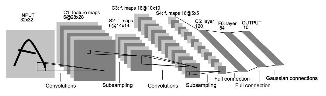
LeNet5 的架构基于这样的观点:图像的特征分布在整张图像上,以及带有可学习参数的卷积是一种用少量参数在多个位置上提取相似特征的有效方式。

在那时候,没有 GPU 帮助训练,甚至 CPU 的速度也很慢。因此,能够保存参数以及计算过程是一个关键进展。这和将每个像素用作一个大型多层神经网络的单独输入相反。

LeNet5 阐述了那些像素不应该被使用在第一层,因为图像具有很强的空间相关性,而使用图像中独立的像素作为不同的输入特征则利用不到这些相关性。

LeNet5特点

LeNet5特征能够总结为如下几点:

1)卷积神经网络使用三个层作为一个系列: 卷积,池化,非线性

2) 使用卷积提取空间特征

3)使用映射到空间均值下采样(subsample)

4)双曲线(tanh)或S型(sigmoid)形式的非线性

5)多层神经网络(MLP)作为最后的分类器

6)层与层之间的稀疏连接矩阵避免大的计算成本

LeNet5实现

1
2
3
4
5
6
7
8
9
10
11
12
13
14
15
16
17
18
19
20
21
22
23
24
25
26
27
28
29
30
31
32
33
34
35
36
37
38
39
40
41
42
43
44
45
46
47
48
49
50
51
52
53
54
55
56
57
58
59
60
61
62
63
64
65
66
67
68
69
70
71
72
73
74
75
76
77
78
79
80
81
82
83
84
85
86
87
88
89
90
91
92
93
94
95
96
97
98
99
100
101
102
103
104
105
106
107
108
109
110
111
112
113
114
115
116
117
118
119
120
121
122
123
124
125
126
127
128
129
130
131
132
133
134
135
136
137
138
139
140
141
142
143
144
145
146
147
148
149
150
151
152
153
154
155
156
157
158
159
160
161
162
163
164
165
166
167
168
169
170
171
172
173
174
175
176
177
178
179
180
181
182
183
184
185
186
187
188
189
190
191
192
193
194
195
196
197
198
199
200
201
202
#!/usr/bin/env python
# -*- coding: utf-8 -*-
# @Time : 2018/8/24 16:35
# @Author : Seven
# @Site :
# @File : LeNet.py
# @Software: PyCharm

# TODO: 0.导入环境

from tensorflow.examples.tutorials.mnist import input_data
import tensorflow as tf
import numpy as np
import random
import matplotlib.pyplot as plt
from sklearn.utils import shuffle
import os
os.environ['TF_CPP_MIN_LOG_LEVEL'] = '2'

# TODO: 1.数据准备

# 使用tensorflow自带的工具加载MNIST手写数字集合
mnist = input_data.read_data_sets('data', reshape=False)

# TODO: 2.数据处理
x_train, y_train = mnist.train.images, mnist.train.labels
x_validation, y_validation = mnist.validation.images, mnist.validation.labels
x_test, y_test = mnist.test.images, mnist.test.labels

# 预先判断下维度是否一致
assert(len(x_train) == len(y_train))
assert(len(x_validation) == len(y_validation))
assert(len(x_test) == len(y_test))

print("Image Shape: {}".format(x_train[0].shape))
print("Training Set: {} samples".format(len(x_train)))
print("Validation Set: {} samples".format(len(x_validation)))
print("Test Set: {} samples".format(len(x_test)))

# TensorFlow预加载的MNIST数据为28x28x1图像。
# 但是,LeNet架构只接受32x32xC图像,其中C是颜色通道的数量。
# 为了将MNIST数据重新格式化为LeNet将接受的形状,我们在顶部和底部填充两行零,并在左侧和右侧填充两列零(28 + 2 + 2 = 32)
x_train = np.pad(x_train, ((0, 0), (2, 2), (2, 2), (0, 0)), 'constant')
x_validation = np.pad(x_validation, ((0, 0), (2, 2), (2, 2), (0, 0)), 'constant')
x_test = np.pad(x_test, ((0, 0), (2, 2), (2, 2), (0, 0)), 'constant')
print("Updated Image Shape: {}".format(x_train[0].shape))

# 查看下灰度图
index = random.randint(0, len(x_train))
image = x_train[index].squeeze()
plt.figure(figsize=(1, 1))
plt.imshow(image, cmap="gray")
# plt.show()
print(y_train[index])

# Shuffle the training data.
x_train, y_train = shuffle(x_train, y_train)

# TODO: 3.准备好placeholder
x = tf.placeholder(tf.float32, (None, 32, 32, 1))
y = tf.placeholder(tf.int32, None)
one_hot_y = tf.one_hot(y, 10)

# TODO: 4.构建网络计算图结构

epochs = 10
batch_size = 128


def LeNet(input):

mu = 0
sigma = 0.1

# 层深度定义
layer_depth = {
'layer1': 6,
'layer2': 16,
'layer3': 120,
'layer_fc1': 84
}

# TODO: 第一层卷积:输入=32x32x1, 输出=28x28x6
conv1_w = tf.Variable(tf.truncated_normal(shape=[5, 5, 1, 6], mean=mu, stddev=sigma))
conv1_b = tf.Variable(tf.zeros(6))

conv1 = tf.nn.conv2d(input, conv1_w, strides=[1, 1, 1, 1], padding='VALID') + conv1_b

# 激活函数
conv1_out = tf.nn.relu(conv1)

# 池化层, 输入=28x28x6, 输出=14x14x6
pool_1 = tf.nn.max_pool(conv1_out, ksize=[1, 2, 2, 1], strides=[1, 2, 2, 1], padding='VALID')
print(pool_1.shape)

# TODO: 第二层卷积: 输入=14x14x6, 输出=10x10x16
conv2_w = tf.Variable(tf.truncated_normal(shape=[5, 5, 6, 16], mean=mu, stddev=sigma))
conv2_b = tf.Variable(tf.zeros(16))

conv2 = tf.nn.conv2d(pool_1, conv2_w, strides=[1, 1, 1, 1], padding='VALID') + conv2_b

# 激活函数
conv2_out = tf.nn.relu(conv2)

# 池化层, 输入=10x10x16, 输出=5x5x16
pool_2 = tf.nn.max_pool(conv2_out, ksize=[1, 2, 2, 1], strides=[1, 2, 2, 1], padding='VALID')

# Flatten 输入=5x5x16, 输出=400
pool_2_flat = tf.reshape(pool_2, [-1, 400])
print(pool_2_flat.shape)

# TODO: 第三层全连接层, 输入=400, 输出=120
fc1_w = tf.Variable(tf.truncated_normal(shape=[400, 120], mean=mu, stddev=sigma))
fc1_b = tf.Variable(tf.zeros(120))

fc1 = tf.matmul(pool_2_flat, fc1_w) + fc1_b

# 激活函数
fc1_out = tf.nn.relu(fc1)
print(fc1_out.shape)

# TODO: 第四层全连接层: 输入=120, 输出=84
fc2_w = tf.Variable(tf.truncated_normal(shape=[120, 84], mean=mu, stddev=sigma))
fc2_b = tf.Variable(tf.zeros(84))

fc2 = tf.matmul(fc1_out, fc2_w) + fc2_b

# 激活函数
fc2_out = tf.nn.relu(fc2)
print(fc2_out.shape)

# TODO: 第五层全连接层: 输入=84, 输出=10
fc3_w = tf.Variable(tf.truncated_normal(shape=[84, 10], mean=mu, stddev=sigma))
fc3_b = tf.Variable(tf.zeros(10))

fc3_out = tf.matmul(fc2_out, fc3_w) + fc3_b
print(fc3_out.shape)

return fc3_out


# TODO: 5.计算损失值并初始化optimizer
learning_rate = 0.001

logits = LeNet(x)
cross_entropy = tf.nn.softmax_cross_entropy_with_logits(logits=logits, labels=one_hot_y)
loss_operation = tf.reduce_mean(cross_entropy)

optimizer = tf.train.AdamOptimizer(learning_rate=learning_rate)
training_operation = optimizer.minimize(loss_operation)

print("FUNCTION READY!!")

# TODO: 6.初始化变量
init = tf.global_variables_initializer()

# TODO: 7.模型评估
correct_prediction = tf.equal(tf.argmax(logits, 1), tf.argmax(one_hot_y, 1))
accuracy_operation = tf.reduce_mean(tf.cast(correct_prediction, tf.float32))


def evaluate(X_data, y_data):
num_examples = len(X_data)
total_accuracy = 0
sess = tf.get_default_session()
for offset in range(0, num_examples, batch_size):
batch_x, batch_y = X_data[offset:offset+batch_size], y_data[offset:offset+batch_size]

accuracy = sess.run(accuracy_operation, feed_dict={x: batch_x, y: batch_y})
total_accuracy += (accuracy * len(batch_x))
return total_accuracy / num_examples


# TODO: 保存模型
saver = tf.train.Saver()


# TODO: 8.训练模型

with tf.Session() as sess:
sess.run(init)
num_examples = len(x_train)

print("Training.....")

for n in range(epochs):
for offset in range(0, num_examples, batch_size):
batch_x, batch_y = x_train[offset:offset+batch_size], y_train[offset:offset+batch_size]
sess.run(training_operation, feed_dict={x: batch_x, y: batch_y})

validation_accuracy = evaluate(x_validation, y_validation)
print("EPOCH {} ...".format(n + 1))
print("Validation Accuracy = {:.3f}".format(validation_accuracy))

saver.save(sess, './model/LeNet.model')
print("Model saved")

print("Evaluate The Model")
# TODO: 读取模型
saver.restore(sess, './model/LeNet.model')
test_accuracy = evaluate(x_test, y_test)
print("Test Accuracy = {:.3f}".format(test_accuracy))

执行结果

1
2
3
4
5
6
7
8
9
10
11
12
13
14
15
16
17
18
19
20
21
22
23
24
25
FUNCTION READY!!
Training.....
EPOCH 1 ...
Validation Accuracy = 0.969
EPOCH 2 ...
Validation Accuracy = 0.974
EPOCH 3 ...
Validation Accuracy = 0.979
EPOCH 4 ...
Validation Accuracy = 0.981
EPOCH 5 ...
Validation Accuracy = 0.984
EPOCH 6 ...
Validation Accuracy = 0.986
EPOCH 7 ...
Validation Accuracy = 0.986
EPOCH 8 ...
Validation Accuracy = 0.986
EPOCH 9 ...
Validation Accuracy = 0.986
EPOCH 10 ...
Validation Accuracy = 0.984
Model saved
Evaluate The Model
Test Accuracy = 0.988

转载请注明:Seven的博客

本文标题:卷积神经网络之LeNet

文章作者:Seven

发布时间:2018年08月24日 - 00:00:00

最后更新:2018年12月11日 - 22:07:15

原始链接:http://yoursite.com/2018/08/24/2018-08-24-DL-CNN-LeNet/

许可协议: 署名-非商业性使用-禁止演绎 4.0 国际 转载请保留原文链接及作者。

------ 本文结束------
坚持原创技术分享,您的支持将鼓励我继续创作!
0%