TensorFlow 从入门到实践
导入TensorFlow模块,查看下当前模块的版本
1 | import tensorflow as tf |
1 | 1.4.0 |
tensorflow是一种图计算框架,所有的计算操作被声明为图(graph)中的节点(Node)
即使只是声明一个变量或者常量,也并不执行实际的操作,而是向图中增加节点
我们来看一上前面安装TensorFlow的时候的测试代码
1 | # 创建名为hello_constant的TensorFlow对象 |
1 | b'Hello World!' |
Tensor
在 TensorFlow 中,数据不是以整数,浮点数或者字符串形式存在的。
这些值被封装在一个叫做 tensor 的对象中。
在 hello_constant = tf.constant(‘Hello World!’) 代码中,
hello_constant是一个 0 维度的字符串 tensor。
tensors 还有很多不同大小:
1 | # A 是一个0维的 int32 tensor |
1 | 1234 |
Session
TensorFlow 的 api 构建在 computational graph(计算图) 的概念上,它是一种对数学运算过程进行可视化的一种方法。让我们把你刚才运行的 TensorFlow 的代码变成一个图:
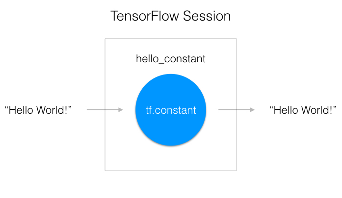
如上图所示,一个 “TensorFlow Session” 是用来运行图的环境。这个 session 负责分配 GPU(s) 和/或 CPU(s) 包括远程计算机的运算。让我们看看怎么使用它:
1 | with tf.Session() as sess: |
这段代码已经从上一行创建了一个 tensor hello_constant。下一行是在session里对 tensor 求值。
这段代码用 tf.Session 创建了一个sess的 session 实例。 sess.run() 函数对 tensor 求值,并返回结果。
constant运算
我们先计算一个线性函数,y=wx+b
1 | w = tf.Variable([[1., 2.]]) |
1 | [[11.9]] |
计算图中所有的数据均以tensor来存储和表达。
tensor是一个高阶张量,二阶张量为矩阵,一阶张量为向量,0阶张量为一个数(标量)。
1 | a = tf.constant(0, name='B') |
1 | print(a) |
1 | Tensor("B:0", shape=(), dtype=int32) |
其他计算操作也同样如此。 tensorflow中的大部分操作都需要通过tf.xxxxx的方式进行调用。
1 | c = tf.add(a,b) |
1 | Tensor("Add_1:0", shape=(), dtype=int32) |
从加法开始, tf.add() 完成的工作与你期望的一样。它把两个数字,两个 tensor,返回他们的和。减法和乘法同样也是直接调用对应的接口函数
1 | x = tf.subtract(10, 4) # 6 |
还有很多关于数学的api,你可以自己去查阅文档
1 | mat_a = tf.constant([[1, 1, 1], [3, 3, 3]]) |
1 | mul_a_b = mat_a * mat_b |
1 | print(mul_a_b) |
1 | Tensor("mul:0", shape=(2, 3), dtype=int32) |
1 | with tf.Session() as sess: |
1 | print(mul_value) |
1 | [[ 2 2 2] |
我们再举几个具体的实例来看看
1 | a = tf.constant(2) |
1 | 5 |
1 | a = tf.constant([2, 2], name='a') |
1 | [[0 2] |
1 | a = tf.constant([[2, 2],[1, 4]], name='a') |
1 | [[ 0 2] |
各式各样的常量
1 | x = tf.zeros([2, 3], tf.int32) |
1 | print(y) |
1 | Tensor("zeros_like:0", shape=(2, 3), dtype=int32) |
1 | with tf.Session() as sess: |
1 | [[0 0 0] |
1 | t_0 = 19 |
1 | [0] |
变量
1 | with tf.variable_scope('meh') as scope: |
例如:求导也是一个运算
1 | x = tf.Variable(2.0) |
1 | [32.0] |
一次性初始化所有变量
1 | my_var = tf.Variable(2, name="my_var") |
1 | 4 |
在前面我们都是采用,先赋值再计算的方法,但是在我们的工作过程中,我会遇到先定义变量,后赋值的情况。
如果你想用一个非常量 non-constant 该怎么办?这就是 tf.placeholder() 和 feed_dict 派上用场的时候了。我们来看看如何向 TensorFlow 传输数据的基本知识。
tf.placeholder()
当你你不能把数据赋值到 x 在把它传给 TensorFlow。因为后面你需要你的 TensorFlow 模型对不同的数据集采取不同的参数。这时你需要 tf.placeholder()!
数据经过 tf.session.run() 函数得到的值,由 tf.placeholder() 返回成一个 tensor,这样你可以在 session 开始跑之前,设置输入。
Session’s feed_dict 功能
1 | x = tf.placeholder(tf.string) |
1 | Hello World |
用 tf.session.run() 里 feed_dict 参数设置占位 tensor。上面的例子显示 tensor x 被设置成字符串 “Hello, world”。当然你也可以用 feed_dict 设置多个 tensor。
placeholder是一个占位符,它通常代表着从外界输入的值。 其中None代表着尚不确定的维度。
1 | input1 = tf.placeholder(tf.float32) |
1 | [array([14.], dtype=float32)] |
把numpy转换成Tensor
1 | import numpy as np |
1 | [[0. 0. 0.] |
类型转换
为了让特定运算能运行,有时会对类型进行转换。例如,你尝试下列代码,会报错:
1 | tf.subtract(tf.constant(2.0),tf.constant(1)) |
1 | TypeError: Input 'y' of 'Sub' Op has type int32 that does not match type float32 of argument 'x'. |
只是因为常量 1 是整数,但是常量 2.0 是浮点数 subtract 需要他们能相符。
在这种情况下,你可以让数据都是同一类型,或者强制转换一个值到另一个类型。这里,我们可以把 2.0 转换成整数再相减,这样就能得出正确的结果:
1 | number = tf.subtract(tf.cast(tf.constant(2.0), tf.int32), tf.constant(1)) |
1 | 1 |
tensorboard 了解图结构/可视化利器
1 | import tensorflow as tf |
1 | 5 |
启动 TensorBoard
在命令端运行:tensorboard –logdir=”./graphs” –port 7007
然后打开Google浏览器访问:http://localhost:7007/
实践
TensorFlow实现线性回归
1 | import numpy as np |
设置生成的图像尺寸和去除警告
1 | os.environ['TF_CPP_MIN_LOG_LEVEL'] = '2' |
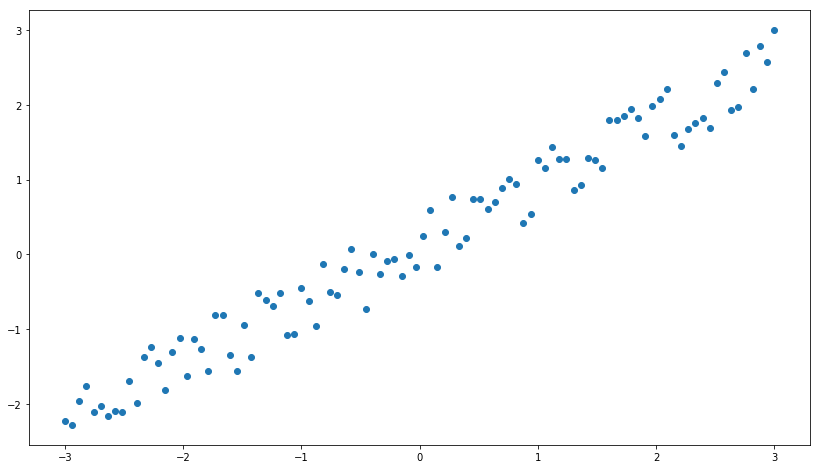
随机生成一个线性的数据,当然你可以换成读取对应的数据集
1 | n_observations = 100 |
准备好placeholder
1 | X = tf.placeholder(tf.float32, name='X') |
初始化参数/权重
1 | W = tf.Variable(tf.random_normal([1]), name='weight') |
计算预测结果
1 | Y_pred = tf.add(tf.multiply(X, W), b) |
计算损失值函数
1 | loss = tf.square(Y - Y_pred, name='loss') |
初始化optimizer
1 | learning_rate = 0.01 |
指定迭代次数,并在session里执行graph
1 | n_samples = xs.shape[0] |
1 | Epoch 0: [0.7908481] |
打印最后更新的w、b的值
1 | print(W, b) |
1 | [0.82705235] [0.16835527] |
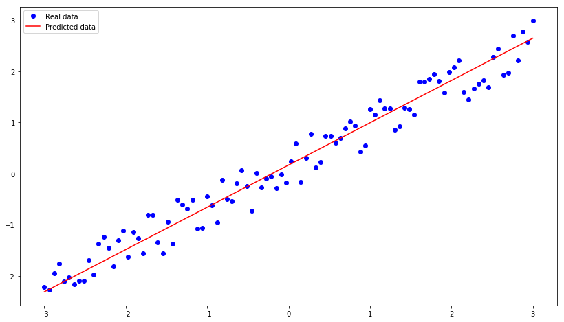
画出线性回归线
1 | plt.plot(xs, ys, 'bo', label='Real data') |
转载请注明:Seven的博客